


★ CODING ★ LISTINGS ★ RSX CIRCLE ★ |
| 3D Graphics (Computing With the Amstrad) | 3D Animated Graphics (Computing With the Amstrad) | 3D Graphics on Amstrad (Popular Computing Weekly) |
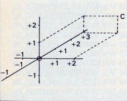
NIGEL SHARP examines the potential for 3D graphic effects from Basic programs 3D VECTOR graphics have been used in several popular Amstrad games — Elite, Starrion and Starstrike to name but a few. Unfortunately, to achieve best effects they have to be written in machine code, involving some very advanced mathematics. However, it is possible to demonstrate the principles of 3D graphics on which these more complicated programs are based, using a Basic program. Program I, for instance, rotates and moves a 3D cube on the screen. The first concept you must get to grips with is 3D coordinates and unless you've forgotten everything you were taught at school, you should know that a point on a graph can be identified by its two coordinates. These are usually called X (horizontal) and Y (vertical). If you look at Figure I you'll see that point A is at (3,2) because it is 3 units to the right of, and two units above, the origin at (0,0). (3,2) can also be written as X=3 and Y=2. Point B is at (-2,1), so X=-2 and Y=1. Notice that X is negative because it is to the left of the origin. Similarly, Y would be negative for a point below the origin. To express this in three dimensions you have the same X and Y coordinates, with the addition of a Z coordinate to indicate how far in front or behind the origin the point is.
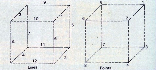
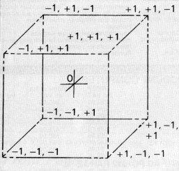
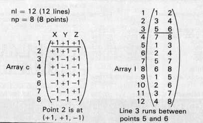
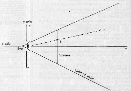
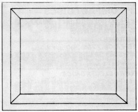
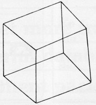
Before the computer can actually draw anything, we must define the object to be drawn, in terms of numbers. As an example how to do this, we will define a cube. First we must allocate a reference number to each point and line on the object, as shown in Figure III. The next step is to work out the 3D coordinates of the object. Figure IV shows you the sort of thing I mean. In Program I the data to describe the object is held in two variables, and two arrays. The number of points and lines are held in the variable np and nl respectively. The array c, dimensioned as c (3,np) holds the X,Y, and Z coordinates of each point. For example c (1,6) is the X coordinate of point 6. The 1 means X, 2 would mean Y, and a 3, Z. The array l, dimensioned as l(2,nl), holds the reference numbers of the two points which the line runs between. Figure V shows the values of nl, np, c, and / for a cube (examples are underlined). This information has been incorporated in DATA between lines 6000 and 6090, and is READ by the routine at line 5000. Now let's move on to the drawing routine. If you take a look at Figure VI you'll see that the eye is at the origin -where the X, Y, and Z axes cross. The X axis is not shown as it runs into and out of the diagram through the eye. The screen is in front of the eye, with the Z axis running through its centre. This means that we must set the graphics origin to the screen centre. We achieve this in line 210 with the command ORIGIN 320,200. Suppose we wish to show the point P on the screen. We draw a line from P to the eye, and where it crosses the screen is where we must plot the point (S in Figure VI). The equations to find the screen coordinates XS and YS of a point in space with 3D coordinates X, Y, Z, are: XS-(X/Z)*M The units used to describe the object are very large compared with the size of screen pixels. The multiplication by M at the end of the equations counteracts this (M is the magnification - a constant found by trial and error, usually about 1000). In our example, both the cube and the eye are at the origin. This is a problem - we will be seeing the cube from inside. We get around this by adding a value (d is used in the program) to the Z coordinate when we draw each point. This has the effect of pushing the cube into the distance. Incidentally, we could not have simply had the coordinates of the cube in the distance in the first place as the rotations, which we will be dealing with shortly, require the object to be centred around the origin. Now you know the basic principles, we can look at the program itself. The routine at line 1000 goes through each line and collects the reference numbers of the points at its two ends, from the array l (lines 1020 and 1030). It then collects the 3D coordinates of these points from the array c (lines 1040 to 1090) and adds d to the Z coordinate to push them into the distance (lines 1100 and 1110). These coordinates are then converted into screen locations (lines 1120 to 1 150) and a line is drawn between them (lines 1160 and 1170). Then the next line is processed until all the lines have been drawn. Now that we have written routines to define and draw the cube, we can actually draw it on the screen. Unfortunately, it isn't very impressive (see Figure VII). What it needs is some movement. Using Basic it won't be very smooth, but we can do our best. There are three ways the cube can be rotated - around the X, Y, or Z axis. Here are the formulae to rotate a point (OX,OY,OZ) to a new point (NX,NY,NZ). SN is the sine of the angle of rotation and CS is the cosine: Rotation around X axis NX=OX Rotation around Y axis Rotation around Z axis Forward and backward movements can be performed by simply increasing and decreasing d. The routines for the three rotations are at lines 2000, 3000, and 4000 respectively. Lines 240 to 370 form the main loop of the program and perform the appropriate rotations as various keys are pressed. The cursor keys, and keys 7 and 9, are for the rotations, while Copy and 8 move the object forwards and backwards. You can see the results of a rotation in Figure VIII. If you are in an adventurous mood after typing in the program, try changing lines 6000 onwards to define some other object. The first two values in line 6010 refer to d and m respectively. You'll probably get away without changing these. If the object is too small, decrease d and/or increase m. If it is too large, increase d and/or decrease m. It is best to keep d above 3 or so. The next two values (line 6020) are the number of points and lines respectively. Following these are the coordinates (grouped into threes for readability) and the line data (grouped in twos). Armed with these principles and using a little thought and patience, you should be able to draw and rotate a variety of interesting shapes.
|