• 
  • A la une du site
  • 100 dernièrs ajouts de fichiers ..
• 
  • Demolist
  • Download
  • Interviews
  • Articles et Dossiers
  • Cheats
  • Gallerie/Musée graphiques
  • Productions CPC+
• 
  • Articles
  • Tests / Gameslist
  • Pokes et Solutions
  • Auteurs
  • Compagnies d'édition
  • Gallerie/Musée graphiques
  • Download
  • Référencement de livres et magazines AMSTRAD CPC
  • Peoples
• 
  • Articles et Chroniques
  • Infos Techniques
  • Crossdev
  • Sources
• 
  • Dépannage
  • Les CPC
  • Les matériel et périphériques
  • Doc's et schémas ...
  • Les montages
  • Service manual
  • Peoples
• 
  • Référencement d'applications AMSTRAD CPC
  • Référencement de livres et magazines AMSTRAD CPC
  • Peoples
• 
  • Download
  • Tools
  • Crossdev
• 

Fractal Landscape Generator (ACU 89/11)

Fractal Landscape Generator (ACU 89/12)

Fractal Landscape Generator (ACU 90/01)

Fractal Landscape Generator (ACU 90/04)

★ Ce texte vous est présenté dans sa version originale ★   ★ This text is presented to you in its original version ★   ★ Este texto se presenta en su versión original ★   ★ Dieser Text wird in seiner Originalfassung präsentiert ★  Learning to landscape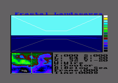 Dean Cracknell delivers the final batch of his three part fractal bonanza. Having produced two programs that calculate the fractal landscape data, we now turn our attention to how the data is to be displayed. The original program used isometric projection to produce a 3D image, but this lacked perspective and did not allow us to see the landscape from different viewing positions. By using these listings you will be able to move around the landscape, and even look underneath. Although the projection uses machine code, the program still takes a couple of minutes to plot, so “flying around the landscape” is the phrase I was trying to avoid here. Perspective and 3D Projection: The machine code in Program 1 pretends that the CPC monitor screen is a window through which you are looking at the fractal landscape. It does this by projecting the landscape onto that window. To illustrate this, look out of a nearby window at the scene on the other side. Sunlight, reflected off the scenery, passes through the glass and enters your eye. Here lenses and light sensitive cells pass the image on to the brain where the most powerful image processing program ever written takes over and we ‘see' the image. If you draw the scene on the glass just as you see it, then this is what the CPC is trying to create on the monitor screen. To achieve this we need to know exactly what the image on the glass would look like. Figure (i) illustrates this: the triangle formed between the viewer, the top of the object and the horizontal has the same proportions as the triangle formed by the viewer and the image on the glass, but a different size. This means that if we divide one of the sides of the larger triangle by one of its other sides, the resulting number will be the same as the same ratio produced by the smaller triangle, or to put it more simply: Height on glass / Distance to glass = Height of object / Distance to object By quickly re-arranging this little equation, it is possible to calculate the height that the object will have on the glass as long as we know all the other numbers, which we do: Hglass = Dglass x Hobject / Dobject This simplified form lacks polish, such as scaling and an offset for the height of the viewer above the ground (his elevation), fully expanded the formula becomes: Hglass = Hscale x Dglass x Elevation-Hobject — / Dobject Normally, the distance from the viewer to the glass will be fixed, so this can be incorporated into the ‘Hscale' constant. Having considered the projection of the height of the object, the width is treated in the same way and produces a similar equation: Xglass = Xscale x Dglass x Xposition-Xobject / Dobject As these two equations are similar, they can be combined into a general purpose equation that can be used for both. The RSX command |PROJECT handles this equation for both the X and H projections. The X and H values come directly from the Fractal data, all the other values are held as variables in the program and can be changed at will. There are limitations to this kind of projection, in that you cannot project the image when the distance from the viewer to the object (Dobject) is zero, as you will get a “Divide by zero” error. In the real, real world this problem is solved by projecting the image into a curved surface, the back of your eye, and then using the brain to compute the true image. The machine code loader of program 1 loads-up the second half of the final machine code, adding a further 15 RSX's to the existing 12. Save and run this program, which will poke the code into memory and save it. The second listing, Program 2, should be typed in as seen, without changing the line numbers and saved as “part-2”. Now you should have a complete version of the full-blown Fractal Landscape Generator, when you run the program, the first landscape will be calculated and displayed as a counter map as before, but now the image display will contain a landscape of sea and sky with three boxes drawn in true perspective, these boxes represent the lowest point, sealevel and the highest point of any landscape, using them as a guide, an idea of where the final image will be can be deduced, pressing [ENTER] or [RETURN] will then draw the full picture. From here on you can move around the landscape using the keys already described or use the new functions added by the latest additions, these new keys are as follows: [O]: Switch On and Off Sea and Sky background. [:]: Changes the Sky/Background colour. [;]: Changes Sea/Horizon colour. The sequence of colours is the same as the colour scale on the right-hand edge of the screen, using SHIFT, the colours step backwards. [ENTER]: Switch between Box-frame and Full Display, for speed, always switch back to Box mode before changing anything (it's quicker). [L]: Multiply Level by 2. Level is the resolution of the projected image, for speed use a lower value, for detail use a higher number, the maximum resolution is 64, which is the resolution of the contor map. [W]: Switch between: Wireframe and Solid image. Wire frame is at least 10 times faster to plot, so use this to adjust your viewing position, then switch to Solid for your final image. [COPY]: Save Projected Frame to disc or tape as file “SO-123.SCR”, where 123 is the frame number. Tape users should press RECORD and PLAY before pressing “COPY”, as tape messages are supressed. [F]: Increase the Frame number by 1, SHIFT 1 decreases the number. [C]: Switch between Contor-Image and Shaded Image for the projected image, in contor mode, the colours are the same as the contor map, in shaded mode the colours are chosen to represent the effect of the sun shining over your left shoulder. [B]: Switch between: Below Sea; Don't Show Sea and Show Sea. These determine how the sea is represented, Don't Show Sea and Show Sea only affect how the Wire-frame image is drawn and look the same in Solid-image. To check that the program ran as expected on a CPC464, I borrowed one and found (to my surprise) that it runs 7,6 faster on a CPC464 than it does on my CPC6128 - does anyone have copies of BASIC V1.0 ROM's to spare? I hope you've all enjoyed this series and may your fractals be fruitful. ACU

CPCrulez[Content Management System] v8.732-desktop/c Page créée en 690 millisecondes et consultée 3756 fois L'Amstrad CPC est une machine 8 bits à base d'un Z80 à 4MHz. Le premier de la gamme fut le CPC 464 en 1984, équipé d'un lecteur de cassettes intégré il se plaçait en concurrent  du Commodore C64 beaucoup plus compliqué à utiliser et plus cher. Ce fut un réel succès et sorti cette même années le CPC 664 équipé d'un lecteur de disquettes trois pouces intégré. Sa vie fut de courte durée puisqu'en 1985 il fut remplacé par le CPC 6128 qui était plus compact, plus soigné et surtout qui avait 128Ko de RAM au lieu de 64Ko.